Labs
- Using the
penguinsdata, - Map
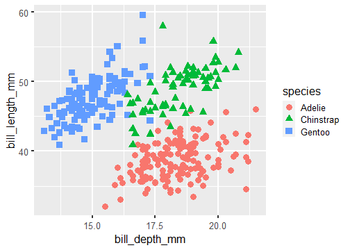
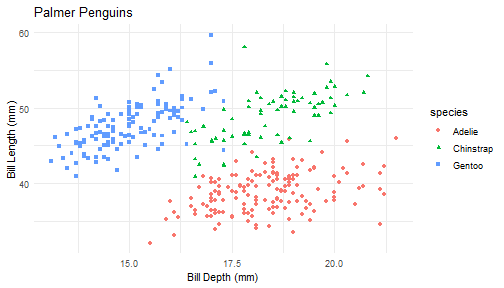
bill depthto x-axis,bill lengthto y-axis,speciesto shape. - Add a layer of points and set the size of the points to 4.
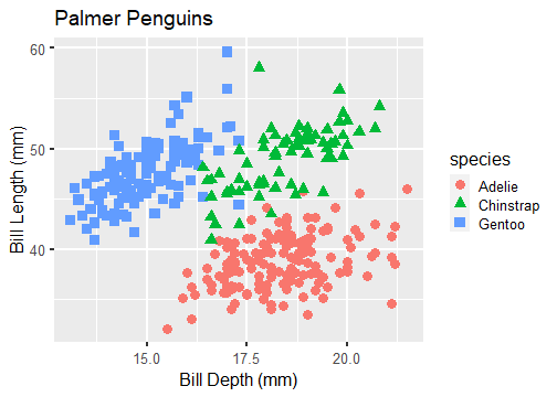
- Add labels to x-axis (Bill Depth(mm)), y-axis (Bill Length(mm)), and the title of the plot (Palmer Penguins).
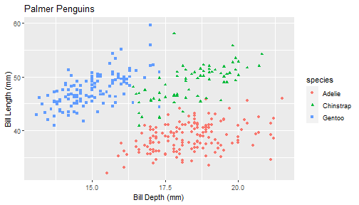
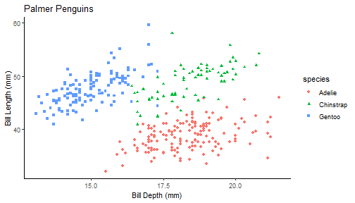
ggplot(penguins, aes(x = bill_depth_mm, y = bill_length_mm, shape = species, color = species)) + geom_point(size = 4) + labs(x = "Bill Depth (mm)", y = "Bill Length (mm)", title = "Palmer Penguins")ggplot(penguins, aes(x = bill_depth_mm, y = bill_length_mm, shape = species, color = species)) + geom_point() + labs(x = "Bill Depth (mm)", y = "Bill Length (mm)", title = "Palmer Penguins") + theme_bw()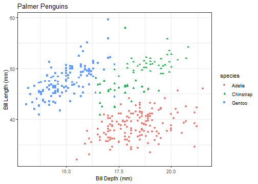
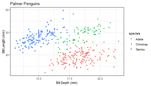
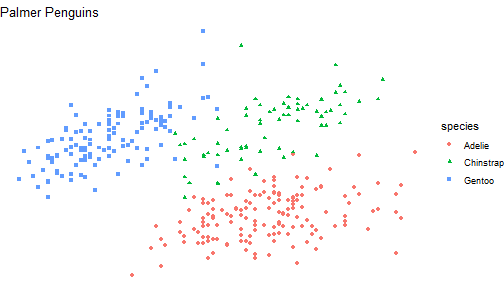
ggplot(penguins, aes(x = bill_depth_mm, y = bill_length_mm, shape = species, color = species)) + geom_point() + labs(x = "Bill Depth (mm)", y = "Bill Length (mm)", title = "Palmer Penguins") + theme_bw() + theme(text = element_text(size=20))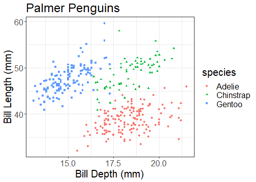
ggplot(penguins, aes(x = bill_depth_mm, y = bill_length_mm, shape = species, color = species)) + geom_point(size = 4) + facet_grid(.~species)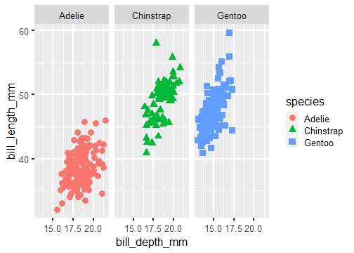
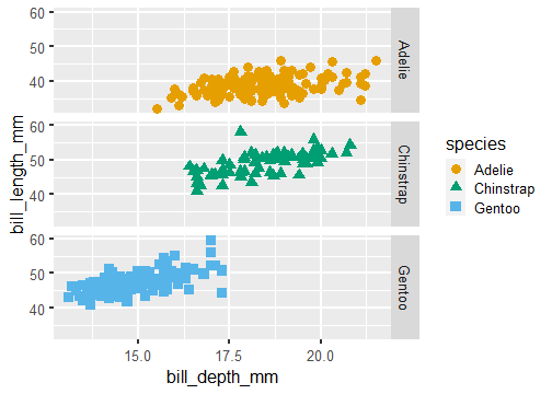
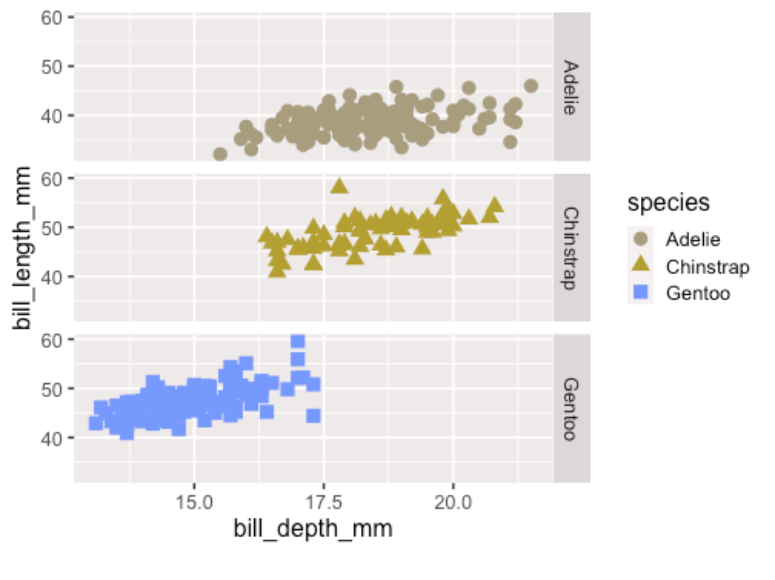
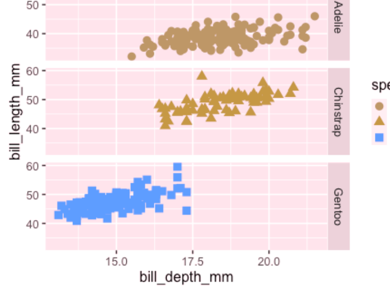
ggplot(penguins, aes(x = bill_depth_mm, y = bill_length_mm, shape = species, color = species)) + geom_point(size = 4) + facet_grid(species~.)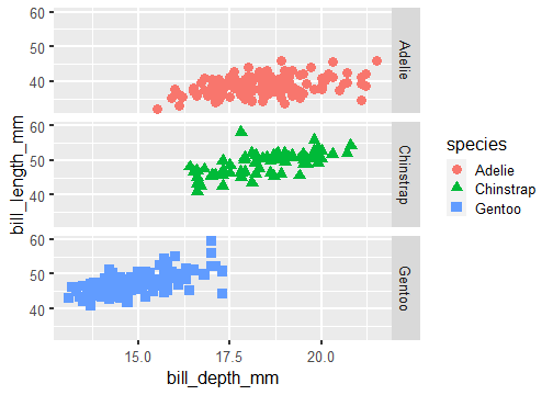
ggplot(penguins, aes(x = bill_depth_mm, y = bill_length_mm)) + geom_point() + xlim(0, 30) + ylim(0, 70)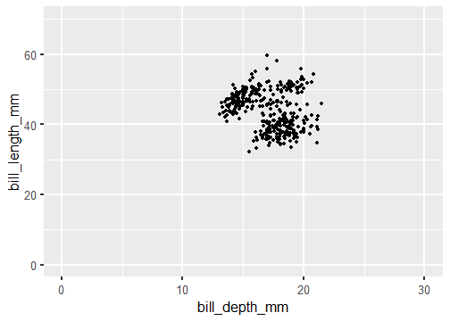
ggplot(data = usa, aes(x = long, y = lat))
ggplot(data = usa, aes(x = long, y = lat)) + geom_polygon()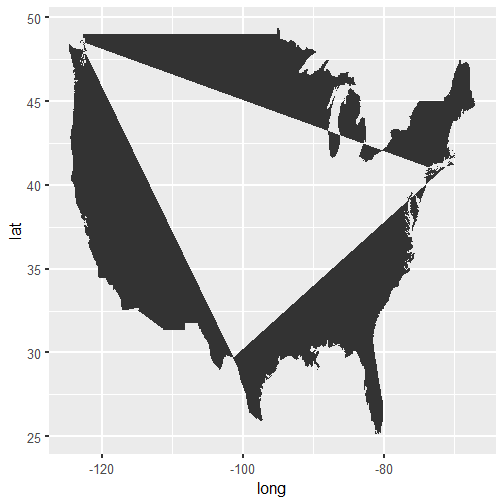
ggplot(data = usa, aes(x = long, y = lat)) + geom_polygon() + coord_fixed(1.4)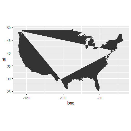
ggplot(data = usa, aes(x = long, y = lat)) + geom_polygon(fill = NA, color = "steelblue") + coord_fixed(1.4)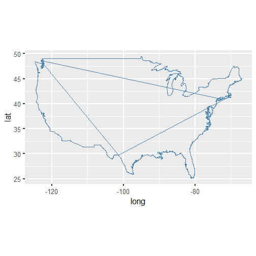
ggplot(data = usa, aes(x = long, y = lat)) + geom_polygon(fill = NA, color = "steelblue", aes(group = group)) + coord_fixed(1.4)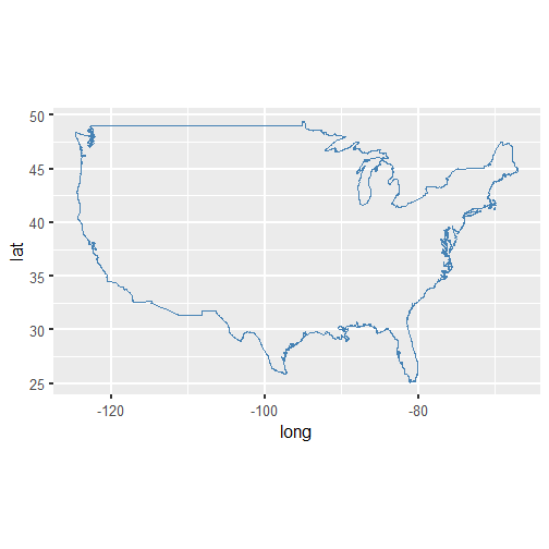
usa_map + geom_point(data = home, aes(x = long, y = lat, color = pop))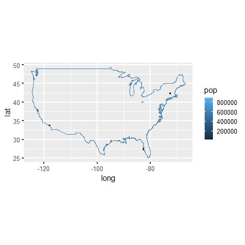
usa_map + geom_point(data = home, aes(x = long, y = lat, size = pop))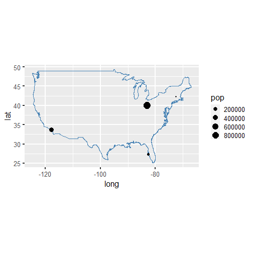
states <- map_data("state")ggplot(data = states, aes(x = long, y = lat, fill = region)) + geom_polygon(aes(group = group)) + coord_fixed(1.4) + guides(fill = "none")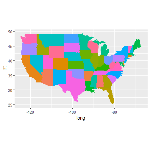
Color blindness simulation: red-blind/protanopia
Color blindness simulation: green-blind/deuteranopia
Color blindness simulation: blue-blind/tritanopia
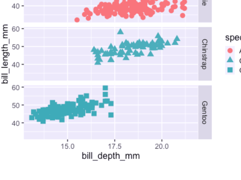
ggplot(penguins, aes(x = bill_depth_mm, y = bill_length_mm, shape = species, color = species)) + geom_point(size = 4) + facet_grid(species~.) + scale_color_manual(values = c("#E69F00", "#009E73", "#56B4E9"))